Quality Control
Once all subjects have processed to completion, it is necessary to perform quality control (QC).
If you used CBRAIN to process your data, you should have already run the QC pipeline by selecting the options for “Launch Claude’s QC script” (as described in Basic Usage of CIVET, CBRAIN Interface - Inputs ). If so, you already have a QC study folder (in our example, “example_QC”) and can proceed to the next section below.
- If you had forgotten to run QC at the same time that you ran CIVET, it is possible to go back and run just QC:
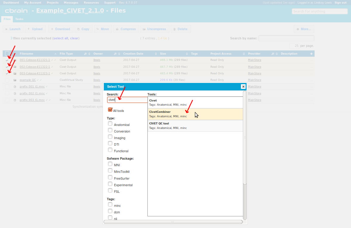
- Under “Files” tab, checkbox all individual Civet Output files, and select “Launch.” Search for “CIVET” in the popup window, and select “CivetCombiner.” This will combine your individual subjects’ output into a single study folder (in our example, “example_QC”).
-
Once CivetCombiner has completed, checkbox your CivetVirtual Study output (“example_QC”), and again select “Launch.” Again, search for “CIVET” in the popup window, but this time select “CIVET QC tool.”
-
It is also possible to view individual subjects’ QC images without running QC as a group; see Basic Usage of CIVET, CBRAIN Interface - Outputs . The images that you can see for each subject when clicking “Show Displayable Contents” may also be viewed by downloading the subject’s output onto your own computer and viewing the
.pngimages within the “verify” directory.
As described in Basic Usage of CIVET, CBRAIN Interface - Outputs , you have a choice of viewing your QC folder output either (1) directly on the CBRAIN interface, or (2) you may download it.
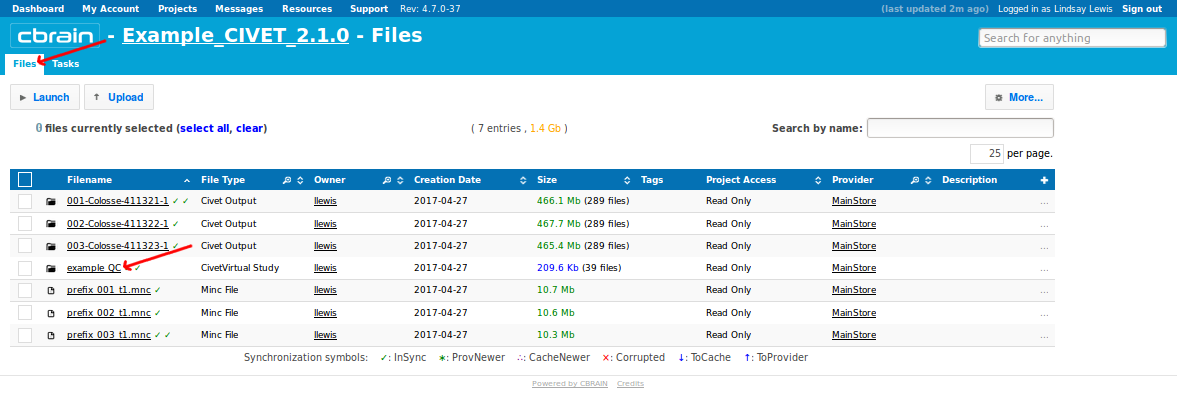
To view it on CBRAIN, navigate to the “Files” tab, and click on the name of your QC study to view all subjects’ QC figures and tables (here, “example_QC”).
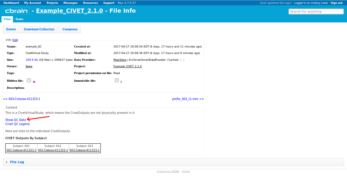
- Click on “Show QC Data.”
If you download it, important files to look for are:
civet_<prefix>.html: main HTML file to load in your web browser, containing group statistics and links to all individual subjects’ QC (verify).pngimagescivet_<prefix>.csv: generic comma-delimited spreadsheet file that can be viewed as a spreadsheet in OpenOffice or Excel, and/or imported with some modifications into SurfStat for analysis (see Statistical-Analyses-Surfstat)
Whether on CBRAIN or from your downloaded files, the HTML table should look roughly like the one below. Various colour codes indicate possible errors; see the legend. The results of red boxed subjects should be examined carefully.
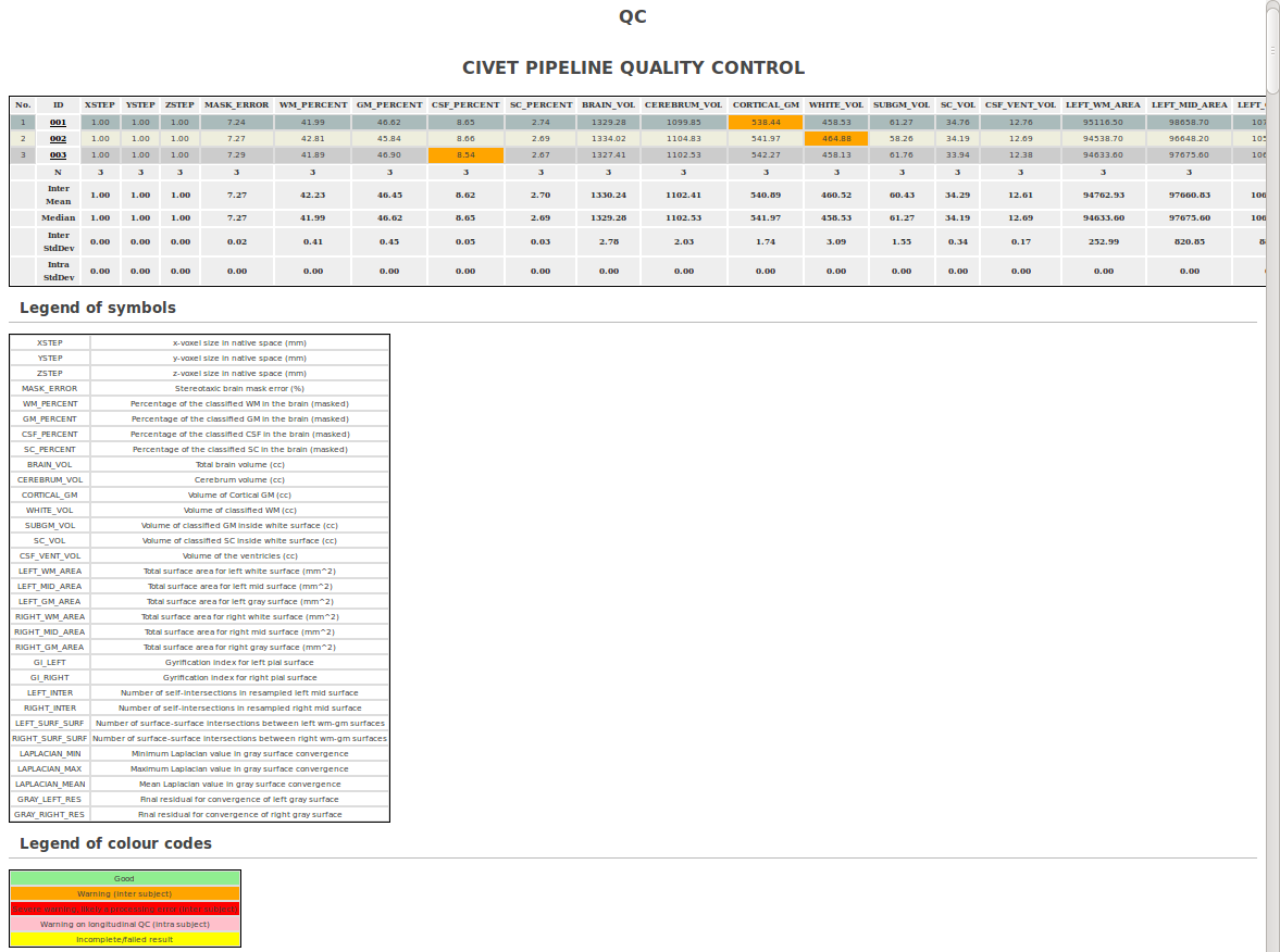
Various metrics are tabulated for the subjects:
XSTEP, YSTEP, ZSTEP: voxel size in native space (mm)MASK_ERROR: error in brain mask in stereotaxic space (difference between subject’s mask and model’s mask), should be 10% or lessWM_PERCENT, GM_PERCENT, CSF_PERCENT: percentages of classified WM, GM, CSF in masked imageBRAIN_VOL: total brain volume in mm3CEREBRUM_VOL: cerebrum volume in mm3CORTICAL_GM: volume of cortical gray matter in mm3 (excludes sub-cortical gray)WHITE_VOL: volume of classified white matter in mm3SUBGM_VOL: volume of classified gray matter inside white surface in mm3SC_VOL: volume of classified SC inside white surface in mm3CSF_VENT_VOL: volume of the ventricles in mm3LEFT_WM_AREA, RIGHT_WM_AREA: total surface area for white surface in mm2LEFT_MID_AREA, RIGHT_MID_AREA: total surface area for mid surface in mm2LEFT_GM_AREA, RIGHT_GM_AREA: total surface area for gray surface in mm2GI_LEFT, GI_RIGHT: gyrification index for left and right gray surfacesLEFT_INTER, RIGHT_INTER: number of self-intersections in left and right resampled mid-surfaces (should be 100 or less)LEFT_SURF_SURF, RIGHT_SURF_SURF: number of surface-surface intersections between white and gray surfaces for left and right hemispheres (values above 500 are often associated with defects due to motion artifacts or masking)LAPLACIAN_MIN, LAPLACIAN_MAX, LAPLACIAN_MEAN: minimum, maximum, and mean Laplacian value in gray surface convergenceGRAY_LEFT_RES,GRAY_RIGHT_RES: final residual for gray surface convergence
At the bottom of this table, the population mean and standard deviation is given for most of these fields. Outliers can be identified by values more than one standard deviation away from the mean, as seen in the plots following the table.
By clicking on the subject id in the table, you can view its verify .png images (same as clicking on “Show Displayable Contents” for each subject on CBRAIN).
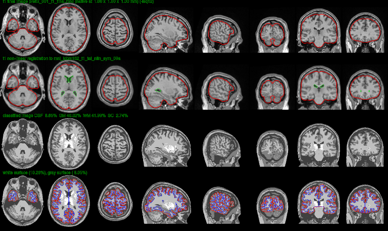
In the verify image below, one looks at the quality of the registration. The first row shows the linearly registered subject, with the red outline representing the border of the brain mask for the stereotaxic model. The subject’s brain should fit tightly inside the red outline for a perfect linear registration. The second row shows the non-linearly transformed subject to the stereotaxic model. The green outline represents the ventricles of the model. If selected for processing, the third row shows the ANIMAL segmentation. The second-to-last row shows the tissue classification while the last row shows the white (blue) and gray (red) cortical surfaces overlaid on top of the tissue classification. The outline of the cortical surfaces should match the tissue classification (zoom in a bit) for complete surface extraction.
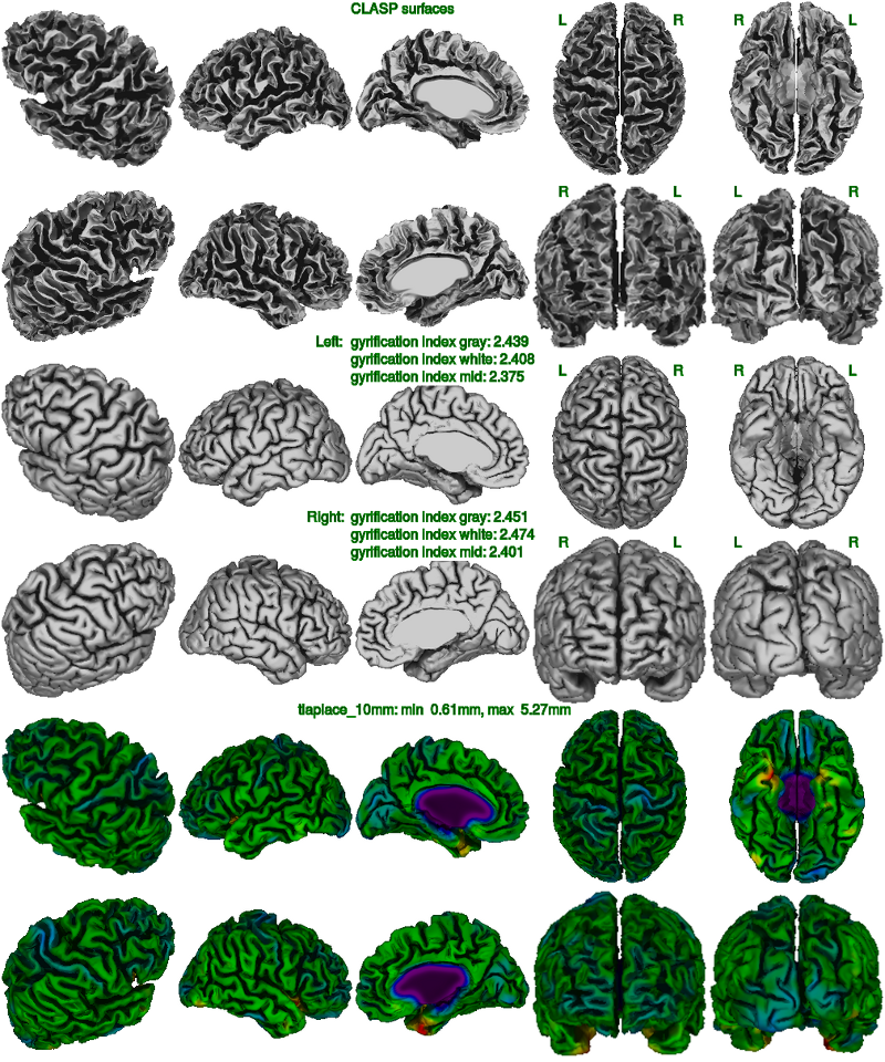
In the clasp image below, one looks at the quality of the surface extraction. (Note: due to maximum size restriction in this web documentation, the resolution of this figure has been reduced.) This figure is helpful to detect masking errors (pieces of skull attached to white surface), motion artifacts (white surface looks jaggy with many bridges across gyri), under-expansion of the gray surface (often in frontal and temporal lobes), as well as poor N3 correction of non-uniformities (atypical pattern of cortical thickness).
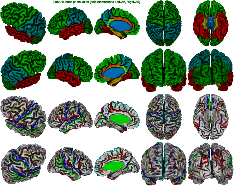
In the basic lobar atlas image below, one looks at the quality of the surface registration. In particular, the border of the frontal and parietal lobes at the central sulcus must be perfectly identified. The AAL and DKT-40 atlas is also available as an option in CIVET; for detailed information on atlases, see VisualGuides. Below the atlas, the painted lines should generally follow the gyri (as opposed to sulci).
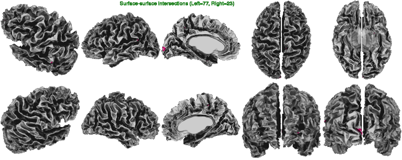
In the surfsurf image below, one looks at the number of gray-white surface-surface intersections (tiny spots in pink). These usually occur when the gray surface is arbitrarily close to the white surface as a result of abnormally thin cortex (usually indicative of poor N3 correction of non-uniformities), of masking errors, of tissue classification errors (often, broken thin strips of white matter in the temporal lobes), and of defects in white surface extraction (erroneous bridge across a sulcus cutting through cortex).
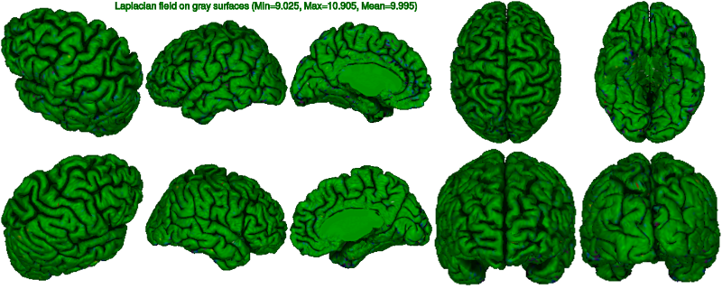
In the laplace figure below, one looks at the convergence of the expansion of the gray surface. A totally green image (Laplacian value of 10) indicates perfect convergence. Colours in high spectrum (red to white) indicate vertices outside the pial surface (over-expansion) while colours in the low spectrum (blue to black) indicate vertices inside the cortex (under-expansion). Using the laplace figure in conjunction with the converg figure below, one can confirm if convergence is incomplete (see example Gray surface (under-)expansion failure)
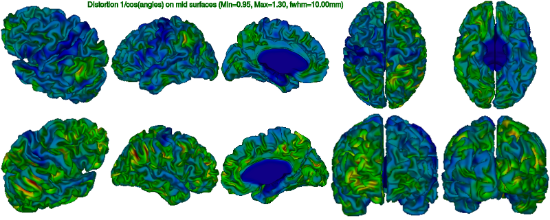
In the angles figure below, one looks at the mesh distortion that occurred during the expansion of the white surface to the gray surface. Ideally, the vertices on the white surface mesh should expand perpendicularly to the gray surface. However, other constraints such as mesh smoothness and mesh self-intersection may cause distortion of the mesh. Large mesh distortion will cause an overestimation of the cortical thickness using the tlink metric. As a quality control tool, very large mesh distortion can also occur in regions where the brain mask is wrong, like extruding into the skull. There is generally greater mesh distortion deep into sulci where many vertices collapse, causing numerical difficulties when evaluating the normal directions.
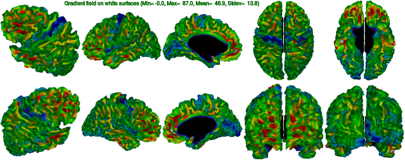
In the gradient figure below, one looks at the magnitude of the gradient of the t1w image (first derivatives) at the vertices of the white surface. During the calibration of the white surface, the position of the white surface is adjusted to the position of the maximum t1w gradient. Notice how the maximum gradient differs deep in sulci and at the top of gyri. The gradient is lowest in the pre-central gyrus where tissue contrast (on a t1w image) is less than in other regions of the brain. The maximum curvature can take on extreme values when the brain mask is wrong.
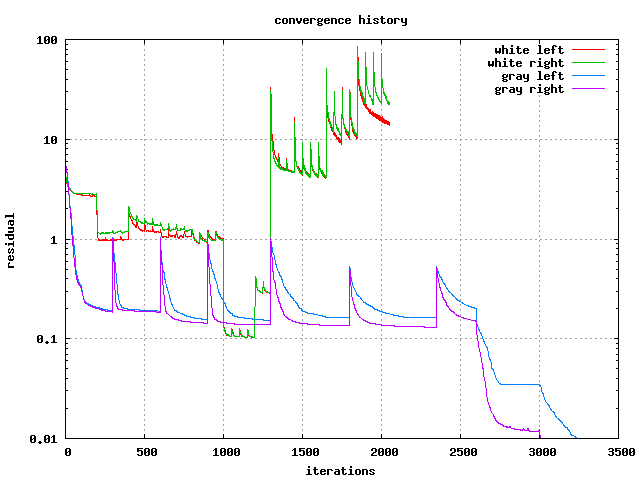
In the converg figure below, one looks at the convergence of the fitting of the white and gray surfaces. The residuals will be very small when the surfaces are very close to the target. From the quality control viewpoint, one looks for incomplete convergence — when convergence stagnates and is represented by a flat line. For gray surfaces, one can confirm, in conjunction with the laplace figure above, that convergence is incomplete (see example Gray surface (under-)expansion failure). For white surfaces, one can confirm, in conjunction with the gradient figure above, that convergence is incomplete. Convergence can be asymmetric.
Examples of QC failure
- Motion artifact failure
- Blood vessel failure
- Inversion failure
- Gray surface (under-)expansion failure (NEW in CIVET 2.1)
Brainbrowser
Brainbrowser allows for visualization of volumes and surfaces through a standard web browser, without the need for specialty software installation.
As described in Basic Usage of CIVET, CBRAIN Interface - Outputs , you may interactively inspect individual subject surfaces and surface overlays using Brainbrowserwithin the CBRAIN interface.
Once you have downloaded your data from CBRAIN, you may also upload individual volumes or surfaces directly into Brainbrowser.
In the event that you suspect motion artifacts, you may wish to use Brainbrowser’s Volume Viewer in order to scroll through your volume ( *.mnc file) to search for potential “ringing.”
Or, you may wish to use the Model Viewer in order to view your surface ( *.obj file) from additional angles.
If you have BIC tools installed, you can also use Display to view your t1 *.mnc with or without its *.obj surfaces overlaid. More information on Display can be found on slides 92–100 here: http://www.bic.mni.mcgill.ca/uploads/Seminars/2014-03-17_-_OMM_Introduction_to_CIVET_2-0_-_Lindsay_Lewis.pdf or MNI Display - Software for Visualization and Segmentation of Surfaces and Volumes